Transform Methods¶

In openAbel there are a couple of different algorithms for the calculation of the Abel transforms implemented, although most of them are just for comparisons and is it recommended to only use the default method.

The main two obstacles when calculating the transforms numerically are the singularity at $r=y$ and the dependence of the result on $y$ , meaning computational complexity is quadratic $O(N^2)$ if one naively integrates. The main difference between the implemented transforms is how those two issues are treated.

When creating the Abel transform object the method keyword argument can be provided to chose different transform methods:

import openAbel
abelObj = openAbel.Abel(nData, forwardBackward, shift, stepSize, method = 3, order = 2)

The methods with end corrections can do the transformation in different orders of accuracy by setting the order keyword argument; all other methods ignore order. Note when we talk about $n$ order accuracy we usually mean $(n+1/2)$ order accuracy due to the square root in the Abel transform kernel. For higher order methods the transformed function has to be sufficiently smooth to achieve the full order of convergence, and in very extreme cases the transform become unstable if high order is used on non-smooth functions. The length of the data vector nData we denote as $N$ in the math formulas.

Overall cases where a user should use anything other than method = 3 (default) and order = 2 (default) to order = 5 will be very rare. For a detailed comparison of the methods it is recommended to look at example004_fullComparison.

Desingularized Trapezoidal Rule¶

# order keyword argument is ignored (only first order implemented)
abelObj = openAbel.Abel(nData, forwardBackward, shift, stepSize, method = 0)

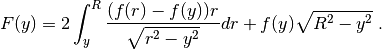
The desingularized trapezoidal rule is probably the simplest practicable algorithm. It subtracts the singularity and integrates it analytically, and numerically integrates the remaining desingularized term with the trapezoidal rule. In the implementation this is done to first order, i.e. for the forward Abel transform this leads to

$F(y)=2\int_{y}^{R}\frac{(f(r)-f(y))r}{\sqrt{r^2-y^2}}dr+f(y)\sqrt{R^2-y^2}\;.$

Now the singularity seems to be removed, but a closer look and one can see that the singularity is still there in the derivative of the integrand, so the convergence is first order in $N$ instead of second order expected when using trapezoidal rule. One can analytically remove the singularity in higher order with more terms, but this gets kinda complicated (and possibly unstable, plus there are other practical issues). The trapezoidal rule portion of the method leads to quadratic $O(N^2)$ computational complexity of the method.

Hansen-Law Method¶

# order keyword argument is ignored (only somewhat first order implemented)
abelObj = openAbel.Abel(nData, forwardBackward, shift, stepSize, method = 1)

The Hansen-Law method by Hansen and Law is a space state model approximation of the Abel transform kernel. With that method recursively transforms a piecewise linear approximation of the input functions to integrate analytically piece by piece. In principle this results in an 2nd order accurate transform, but the approximation of the Abel transform kernel as a sum of exponentials is quite difficult. In other words the approximation

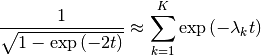
$\frac{1}{\sqrt{1-\exp{(-2t)}}}\approx\sum_{k=1}^K\exp{(-\lambda_kt)}$

is in practice not possible to achieve with high accuracy and reasonable $K$ . This is the main limitation of the method, and the original space state model approxmation has a typical relative error of $10^{-3}$ at best – then it just stops converging with increasing $N$ . If one ignores several details that makes the method apparently linear $O(N)$ computational complexity, so it is implemented here for comparisons. More comments in the remarks.

Trapezoidal Rule with End Corrections¶

# 0 < order < 20
abelObj = openAbel.Abel(nData, forwardBackward, shift, stepSize, method = 2, order = 2)

The trapezoidal rule with end correction improves on the desingularized trapezoidal rule. It doesn’t require analytical integration because it uses precalculated end correction coefficients of arbitrary order. As described in Kapur one can contruct $\alpha_i$ and $\beta_i$ such that the approxmation

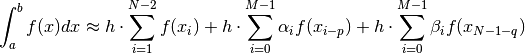
$\int_{a}^{b}f(x)dx \approx h\cdot\sum_{i=1}^{N-2}f(x_i) + h\cdot\sum_{i=0}^{M-1}\alpha_if(x_{i-p}) + h\cdot\sum_{i=0}^{M-1}\beta_if(x_{N-1-q})$

is accurate to order $M$ . Note that $p$ and $q$ should be chosen such that the correction is centered around the end points: Similar to central finite differences this leads to an arbitrary order stable scheme, and thus incredibly fast convergence and small errors. Otherwise it’s not recommended to go higher than $M=5$ , again similar to forward and backward finite differences. The trapezoidal rule portion of the method leads to quadratic $O(N^2)$ computational complexity of the method.

Since the calculation of the end correction coefficients requires some analytical calculations, is quite troublesome and time consuming, they have been precalculated in Mathematica and stored in binary *.npy , so they are only loaded by the openAbel code when needed and don’t have to be calculated. The *Mathematica* notebook which was used to calculate these end correction coefficients can be found in this repository as well.

Fast Multipole Method with End Corrections¶

# 0 < order < 20
abelObj = openAbel.Abel(nData, forwardBackward, shift, stepSize, method = 3, order = 2)

The default and recommended method is the Fast Multipole Method (FMM) with end corrections. This method provides a fast linear $O(N)$ computational complexity transform of arbitrary order. The specific FMM used is based on Chebyshev interpolation and nicely described and applied by Tausch on a similar problem. In principle the FMM uses a hierarchic decomposition to combine a linear amount of direct short-range contributions and smooth approximations of long-range contributions with efficient reuse of intermediate results to get in total a linear $O(N)$ computational complexity algorithm. This method thus provides extremely fast convergence and fast computation, and is optimal in that sense for the intended purpose.

Remarks on Transforms of Noisy Data¶

For specifically the inverse Abel transform of noisy data (e.g. experimental data) there are a lot of algorithms described in literature which might perform better in some aspects, since they either incorporate some assumptions about the data or some kind of smoothing/filtering of the noise. A nice starting point for people interested in those methods is the Python module PyAbel.

However, there is no reason not to combine the methods provided in openAbel with some kind of filering for nicer results. I’ve had good results with maximally flat filters, as seen in example003_noisyBackward, and with additional material in the Mathematica notebook.

Overall even in this special case there are no algorithms to my knowledge which perform inherently better than the default algorithms of openAbel by default.