example004_fullComparison
This example provides a rather extensive comparison of different openAbel methods. It shows how well the main methods perform in every regard, especially if the input data is sufficiently smooth. Most importantly one can see the fast convergence of the higher order methods in the bottom left plot, and the linear computational complexity of the main methods in the bottom middle and right plots.
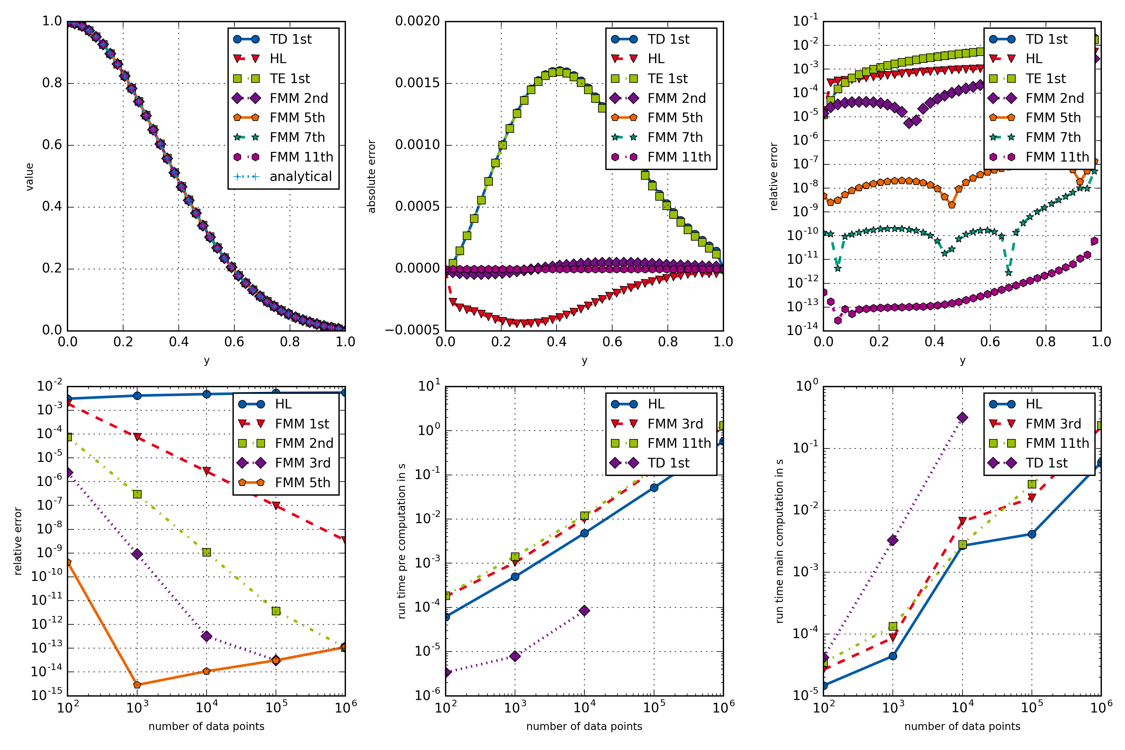
Comparison of different openAbel methods.
1 2 3 4 5 6 7 8 9 10 11 12 13 14 15 16 17 18 19 20 21 22 23 24 25 26 27 28 29 30 31 32 33 34 35 36 37 38 39 40 41 42 43 44 45 46 47 48 49 50 51 52 53 54 55 56 57 58 59 60 61 62 63 64 65 66 67 68 69 70 71 72 73 74 75 76 77 78 79 80 81 82 83 84 85 86 87 88 89 90 91 92 93 94 95 96 97 98 99 100 101 102 103 104 105 106 107 108 109 110 111 112 113 114 115 116 117 118 119 120 121 122 123 124 125 126 127 128 129 130 131 132 133 134 135 136 137 138 139 140 141 142 143 144 145 146 147 148 149 150 151 152 153 154 155 156 157 158 159 160 161 162 163 164 165 166 167 168 169 170 171 172 173 174 175 176 177 178 179 180 181 182 183 184 185 186 187 188 189 190 191 192 193 194 195 196 197 198 199 200 201 202 203 204 205 206 207 208 209 210 211 212 213 214 215 216 217 | ############################################################################################################################################
# Example to showcase the different methods and orders, including convergence study and run times.
# Forward transform is done here, but similar results apply to the backward transform.
# This example takes possibly minutes to run, so beware
############################################################################################################################################
import openAbel as oa
import numpy as np
from scipy.special import erf
import matplotlib.pyplot as mpl
import datetime as dt
import time as ti
############################################################################################################################################
# Plotting setup
params = {
'axes.labelsize': 8,
'font.size': 8,
'legend.fontsize': 10,
'xtick.labelsize': 10,
'ytick.labelsize': 10,
'text.usetex': False,
'figure.figsize': [12., 8.]
}
mpl.rcParams.update(params)
# Color scheme
colors = ['#005AA9','#E6001A','#99C000','#721085','#EC6500','#009D81','#A60084','#0083CC','#F5A300','#C9D400','#FDCA00']
# Plot markers
markers = ["o", "v" , "s", "D", "p", "*", "h", "+", "^", "x"]
# Line styles
linestyles = ['-', '--', '-.', ':','-', '--', '-.', ':','-', '--', '-.', ':']
lw = 2
fig, ((ax1, ax2, ax3), (ax4, ax5, ax6)) = mpl.subplots(2, 3)
############################################################################################################################################
# Error over radius of different methods and orders
def errorAbel(nData, method, order):
dx = 1./(nData-1);
xx = np.linspace(0., 1., nData)
sig = 1./3.
dataIn = 1./sig/np.sqrt(2*np.pi)*np.exp(-0.5*xx**2/sig**2)
dataAna = 2.*1./sig/np.sqrt(2*np.pi)*np.exp(-0.5*xx**2/sig**2) * \
np.sqrt(np.pi/2.)*sig*erf(np.sqrt(1**2-xx**2)/np.sqrt(2.)/sig)
abelObj = oa.Abel(nData, -1, 0., dx, method = method, order = order)
dataOut = abelObj.execute(dataIn)
abserr = dataOut-dataAna
relerr = np.abs(abserr/np.clip(dataAna, 1.e-300, None))
return (xx, abserr, relerr, dataOut, dataAna)
# Loop over several methods and orders
names = ['TD 1st', 'HL', 'TE 1st', 'FMM 2nd', 'FMM 5th', 'FMM 7th', 'FMM 11th']
orders = [-1, -1, 1, 2, 5, 7, 11]
methods = [0, 1, 2, 3, 3, 3, 3]
for ii in range(len(orders)):
(xx, abserr, relerr, dataOut, dataAna) = errorAbel(40, methods[ii], orders[ii])
ax1.plot(xx, dataOut, label = str(names[ii]), color = colors[ii],
linestyle = linestyles[ii], marker = markers[ii], linewidth=lw)
ax2.plot(xx, abserr, label = str(names[ii]), color = colors[ii],
linestyle = linestyles[ii], marker = markers[ii], linewidth=lw)
ax3.semilogy(xx[:-1], relerr[:-1], label=str(names[ii]), color = colors[ii],
linestyle = linestyles[ii], marker = markers[ii], linewidth=lw)
ii += 1
ax1.plot(xx, dataAna, label = 'analytical', color = colors[ii],
linestyle = linestyles[ii], marker = markers[ii], linewidth=lw)
ax1.legend()
ax1.set_xlabel('y')
ax1.set_ylabel('value')
ax1.grid(True)
ax2.legend()
ax2.set_xlabel('y')
ax2.set_ylabel('absolute error')
ax2.grid(True)
ax3.legend()
ax3.set_xlabel('y')
ax3.set_ylabel('relative error')
ax3.grid(True)
############################################################################################################################################
# Convergence of different methods and orders
def convergenceAbel(nArray, method, order):
conv = np.empty(nArray.shape[0])
for ii in range(nArray.shape[0]):
nData = nArray[ii]
dx = 1./(nData-1);
xx = np.linspace(0., 1., nData)
sig = 1./3.
dataIn = 1./sig/np.sqrt(2*np.pi)*np.exp(-0.5*xx**2/sig**2)
abelObj = oa.Abel(nData, -1, 0., dx, method = method, order = order)
dataOut = abelObj.execute(dataIn)
dataAna = 2./sig/np.sqrt(2*np.pi)*np.exp(-0.5*xx**2/sig**2) * \
np.sqrt(np.pi/2.)*sig*erf(np.sqrt(1**2-xx**2)/np.sqrt(2.)/sig)
conv[ii] = np.sqrt(np.sum(((dataOut-dataAna)/np.clip(dataAna, 1.e-300, None))**2)/nData)
return conv
# Loop over several methods and orders
names = ['HL', 'FMM 1st', 'FMM 2nd', 'FMM 3rd', 'FMM 5th']
orders = [-1, 1, 2, 3, 5]
methods = [1, 3, 3, 3, 3]
nArray = 10**(np.arange(5)+2)
for ii in range(len(orders)):
conv = convergenceAbel(nArray, methods[ii], orders[ii])
ax4.loglog(nArray, conv, label=str(names[ii]), color = colors[ii],
linestyle = linestyles[ii], marker = markers[ii], linewidth=lw)
ax4.legend()
ax4.set_xlabel('number of data points')
ax4.set_ylabel('relative error')
ax4.grid(True)
############################################################################################################################################
# Run times of different methods and orders
def runtimesAbel(nArray, nMeasure, method, order):
runtimes = np.zeros(nArray.shape[0])
runtimesPre = np.zeros(nArray.shape[0])
for ii in range(nArray.shape[0]):
dataIn = np.ones(nArray[ii])
T = np.empty(nMeasure)
for jj in range(nMeasure):
t0 = ti.time()
abelObj = oa.Abel(nArray[ii], -1, 0., 1., method = method, order = order)
t1 = ti.time()
T[jj] = t1-t0
runtimesPre[ii] = np.sum(T)/nMeasure
abelObj = oa.Abel(nArray[ii], -1, 0., 1., method = method, order = order)
t0 = ti.time()
for jj in range(nMeasure):
dataOut = abelObj.execute(dataIn)
t1 = ti.time()
runtimes[ii] = (t1-t0)/nMeasure
return (runtimesPre, runtimes)
# Loop over several methods and orders
names = ['HL', 'FMM 3rd', 'FMM 11th', 'TD 1st']
orders = [-1, 3, 11, -1]
methods = [1, 3, 3, 0]
nArray = 10**(np.arange(5)+2)
nArraySmall = 10**(np.arange(3)+2)
for ii in range(3):
(runtimesPre, runtimes) = runtimesAbel(nArray, 5, methods[ii], orders[ii])
ax5.loglog(nArray, runtimesPre, label=str(names[ii]), color = colors[ii],
linestyle = linestyles[ii], marker = markers[ii], linewidth=lw)
ax6.loglog(nArray, runtimes, label=str(names[ii]), color = colors[ii],
linestyle = linestyles[ii], marker = markers[ii], linewidth=lw)
for ii in range(3,len(names)):
(runtimesPre, runtimes) = runtimesAbel(nArraySmall, 5, methods[ii], orders[ii])
ax5.loglog(nArraySmall, runtimesPre, label=str(names[ii]), color = colors[ii],
linestyle = linestyles[ii], marker = markers[ii], linewidth=lw)
ax6.loglog(nArraySmall, runtimes, label=str(names[ii]), color = colors[ii],
linestyle = linestyles[ii], marker = markers[ii], linewidth=lw)
ax5.legend()
ax5.set_xlabel('number of data points')
ax5.set_ylabel('run time pre computation in s')
ax5.grid(True)
ax6.legend()
ax6.set_xlabel('number of data points')
ax6.set_ylabel('run time main computation in s')
ax6.grid(True)
mpl.tight_layout()
mpl.savefig('example004_fullComparison.png', dpi=300)
mpl.show()
|