example002_methodOrder
This example shows how to switch to other transform methods and orders. It illustrates how quickly the errors of high order methods converge to machine precision, even for very small data sets. It is of course important that the input data is sufficiently smooth and other errors (e.g. truncation errors) are small enough as well.
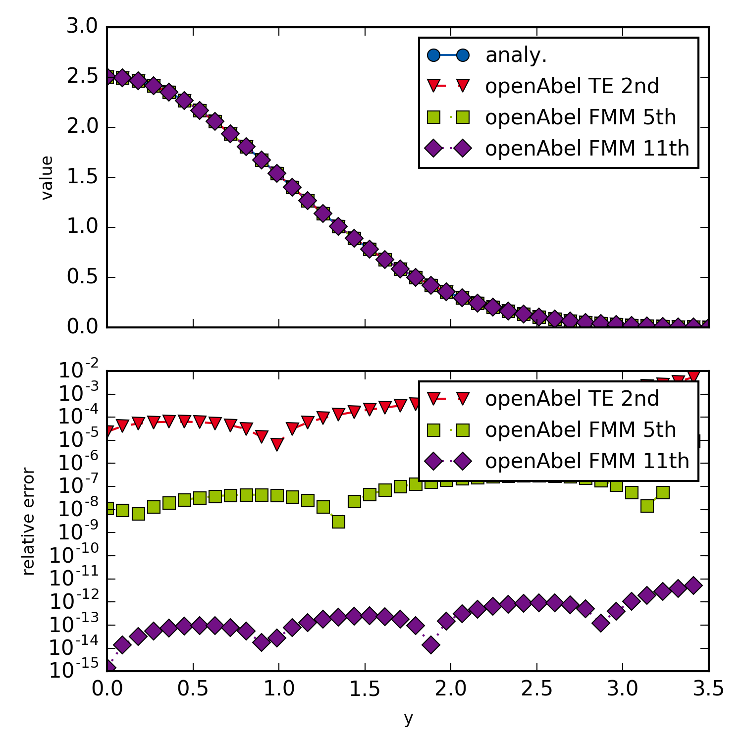
Different methods and orders.
1 2 3 4 5 6 7 8 9 10 11 12 13 14 15 16 17 18 19 20 21 22 23 24 25 26 27 28 29 30 31 32 33 34 35 36 37 38 39 40 41 42 43 44 45 46 47 48 49 50 51 52 53 54 55 56 57 58 59 60 61 62 63 64 65 66 67 68 69 70 71 72 73 74 75 76 77 78 79 80 81 82 83 84 85 86 87 88 89 90 91 92 93 | ############################################################################################################################################
# Simple example which shows how to select different methods and orders.
# Results are compared with the analytical solution.
############################################################################################################################################
import openAbel
import numpy as np
from scipy.special import erf
import matplotlib.pyplot as mpl
############################################################################################################################################
# Plotting setup
# This block can be ignored, it's just for nicer plots.
params = {
'axes.labelsize': 8,
'font.size': 8,
'legend.fontsize': 10,
'xtick.labelsize': 10,
'ytick.labelsize': 10,
'text.usetex': False,
'figure.figsize': [5., 5.]
}
mpl.rcParams.update(params)
# Color scheme
colors = ['#005AA9','#E6001A','#99C000','#721085','#EC6500','#009D81','#A60084','#0083CC','#F5A300','#C9D400','#FDCA00']
# Plot markers
markers = ["o", "v" , "s", "D", "p", "*", "h", "+", "^", "x"]
# Line styles
linestyles = ['-', '--', '-.', ':','-', '--', '-.', ':','-', '--', '-.', ':']
lw = 2
############################################################################################################################################
# Parameters
nData = 40
shift = 0.
xMax = 3.5
sig = 1.
stepSize = xMax/(nData-1)
forwardBackward = -1 # Forward transform, similar definition ('1' = backward) as in FFT libraries.
# Create Abel transform object for three different methods and orders.
# Some methods ignore the order keyword argument, and for the normal user
# only method = 3 and order = 2 to order = 5 are recommended.
# Higher orders require data outside the integration domain to be stable.
# For more information see the documentation.
abelObj0 = openAbel.Abel(nData, forwardBackward, shift, stepSize, method = 2, order = 2)
abelObj1 = openAbel.Abel(nData, forwardBackward, shift, stepSize, method = 3, order = 5)
abelObj2 = openAbel.Abel(nData, forwardBackward, shift, stepSize, method = 3, order = 11)
# Input data
xx = np.linspace(shift*stepSize, xMax, nData)
dataIn = np.exp(-0.5*xx**2/sig**2)
xxExt = np.linspace(shift*stepSize, xMax+5*stepSize, nData+5) # floor((order-1)/2) extra points at right end
dataInExt = np.exp(-0.5*xxExt**2/sig**2)
# Backward transform and analytical result
dataOut0 = abelObj0.execute(dataIn)
dataOut1 = abelObj1.execute(dataIn)
dataOut2 = abelObj2.execute(dataInExt, leftBoundary = 2, rightBoundary = 3) # 2 means use even symmetry, 3 means input extra points.
dataOutAna = dataIn*np.sqrt(2*np.pi)*sig*erf(np.sqrt((xMax**2-xx**2)/2)/sig)
# Plotting
fig, axarr = mpl.subplots(2, 1, sharex=True)
axarr[0].plot(xx, dataOutAna, color = colors[0], marker = markers[0], linestyle = linestyles[0], label='analy.')
axarr[0].plot(xx, dataOut0, color = colors[1], marker = markers[1], linestyle = linestyles[1], label='openAbel TE 2nd')
axarr[0].plot(xx, dataOut1, color = colors[2], marker = markers[2], linestyle = linestyles[2], label='openAbel FMM 5th')
axarr[0].plot(xx, dataOut2, color = colors[3], marker = markers[3], linestyle = linestyles[3], label='openAbel FMM 11th')
axarr[0].set_ylabel('value')
axarr[0].legend()
axarr[1].semilogy(xx[:-1]/sig, np.abs((dataOut0[:-1]-dataOutAna[:-1])/dataOutAna[:-1]),
color = colors[1], marker = markers[1], linestyle = linestyles[1], label = 'openAbel TE 2nd')
axarr[1].semilogy(xx[:-1]/sig, np.abs((dataOut1[:-1]-dataOutAna[:-1])/dataOutAna[:-1]),
color = colors[2], marker = markers[2], linestyle = linestyles[2], label='openAbel FMM 5th')
axarr[1].semilogy(xx[:-1]/sig, np.abs((dataOut2[:-1]-dataOutAna[:-1])/dataOutAna[:-1]),
color = colors[3], marker = markers[3], linestyle = linestyles[3], label='openAbel FMM 11th')
axarr[1].set_ylabel('relative error')
axarr[1].set_xlabel('y')
axarr[1].legend()
mpl.tight_layout()
mpl.savefig('example002_methodOrder.png', dpi=300)
mpl.show()
|